Module 1.1 - Learning With Derivatives
Training Data
- Set of datapoints, each $(x,y)$
- $x$ position $x_1, x_2$
- $y$ true label, color
In [2]:
split_graph(s1, s2)
Out[2]:
In [3]:
def forward(self, x1: float, x2: float) -> float:
    return self.w1.value * x1 + self.w2.value * x2 + self.b.value
Graphical Notation
- Red is more positive, blue is more negative.
- $m(x)$ provides a value for every $x_1, x_2$ every point.
- Line represents seperator
Model 1
- Linear Model
In [4]:
from minitorch import Parameter, Module
class Linear(Module):
    def __init__(self, w1, w2, b):
        super().__init__()
        self.w1 = Parameter(w1)
        self.w2 = Parameter(w2)
        self.b = Parameter(b)

    def forward(self, x1: float, x2: float) -> float:
        return self.w1.value * x1 + self.w2.value * x2 + self.b.value
Decision Boundary: Model 1
In [5]:
model = Linear(w1=1, w2=1, b=-0.9)
draw_graph(model)
Out[5]:
Distance Determines Fit
- $m(x)$ red or blue.
In [6]:
with_points(s1, s2, Linear(1, 1, -0.4))
Out[6]:
Point Loss
In [8]:
graph(point_loss, [], [])
Out[8]:
In [9]:
graph(point_loss, [], [-2, -0.2, 1])
Out[9]:
!-- #endregion -->
Warmup: ReLU
In [10]:
def point_loss(m_x):
    return minitorch.operators.relu(m_x)
In [11]:
graph(point_loss, [], [])
Out[11]:
Loss
- $L(\theta)$ loss is a function of parameters
- We change parameters, decision boundary changes
Lecture Quiz
Outline
- Model Fit
- Symbolic Derivatives
- Numerical Derivatives
- Module 1
Model Fitting
Class Goal
- Find parameters that minimize loss
In [12]:
hcat(
    [show(Linear(1, 1, -0.6)), show(Linear(1, 1, -0.7)), show(Linear(1, 1, -0.8))], 0.3
)
Out[12]:
Numerical Optimization
- Many, many different approaches
- Our focus: gradient descent
- Workhorse of modern machine learning
Iterative Parameter Fitting
- Compute the loss function, $L(\theta)$
- See how small changes would change the loss
- Update to parameters to locally reduce the loss
Example: Update Bias
In [13]:
model1 = Linear(w1=1, w2=1, b=-0.4)
model2 = Linear(w1=1, w2=1, b=-0.5)
In [14]:
compare(model1, model2)
Out[14]:
Step 1: Compute Loss
In [15]:
with_points(s1, s2, Linear(1, 1, -1.5))
Out[15]:
In [16]:
def point_loss(out, y=1):
    return y * -math.log(  # Correct Side
        minitorch.operators.sigmoid(-out)  # Log-Sigmoid
    )  # Distance
Loss
In [17]:
def full_loss(m):  # Given m( ; \theta)
    l = 0
    for x, y in zip(s.X, s.y):  # For all training data
        l += point_loss(-m.forward(*x), y)
    return -l
In [18]:
hcat(
    [
        graph(point_loss, [], [-2, -0.2, 1]),
        graph(lambda x: point_loss(-x), [-1, 0.4, 1.3], []),
    ],
    0.3,
)
Out[18]:
Step 2: Find Direction of Improvement
In [19]:
hcat([show(Linear(1, 1, -1.5)), show(Linear(1, 1, -1.45))], 0.3)
Out[19]:
Step 3: Update Parameters Iteratively
In [20]:
set_svg_height(300)
show_loss(full_loss, Linear(1, 1, 0))
Out[20]:
Our Challenge
How do we find the right direction?
Symbolic Derivatives
Review: What is a Derivative?
How small changes in input impact output.
- $f(x)$ - function
- $x$ - point
- $f'(x)$ - "rise/run"
Review: Derivative
$$f(x) = x^2 + 1$$
In [21]:
def f(x):
    return x * x + 1.0


plot_function("f(x)", f)
Review: Derivative
$$f(x) = x^2 + 1$$ $$f'(x) = 2x$$
In [22]:
def f_prime(x):
    return 2 * x


def tangent_line(slope, x, y):
    def line(x_):
        return slope * (x_ - x) + y

    return line


plot_function("f(x) vs f'(2)", f, fn2=tangent_line(f_prime(2), 2, f(2)))
Symbolic Derivative
- Standard high-school derivatives
- Rewrite $f$ to new form $f'$
- Produces mathematical function
Example Function
$$f(x) = \sin(2 x)$$
In [23]:
plot_function("f(x) = sin(2x)", lambda x: math.sin(2 * x))
Symbolic Derivative
$$f(x) = \sin(2 x) \Rightarrow f'(x) = 2 \cos(2 x)$$
In [24]:
plot_function(
    "f'(x) = 2*cos(2x)", lambda x: 2 * math.cos(2 * x), fn2=lambda x: math.sin(2 * x)
)
Multiple Arguments
$$f(x, y) = \sin(x) + \cos(y)$$
In [25]:
plot_function3D(
    "f(x, y) = sin(x) + 2 * cos(y)", lambda x, y: math.sin(x) + 2 * math.cos(y)
)
Derivatives with Multiple Arguments
$$f_x'(x, y) = \cos(x) \ \ \ f_y'(x, y) = -2 \sin(y)$$
In [26]:
plot_function3D("f'_x(x, y) = cos(x)", lambda x, y: math.cos(x))
Numerical Derivatives
In [27]:
def f(x: float) -> float: ...
Derivative as higher-order function
$$f(x) = ...$$ $$f'(x) = ...$$
In [28]:
def derivative(f: Callable[[float], float]) -> Callable[[float], float]:
    def f_prime(x: float) -> float: ...

    return f_prime
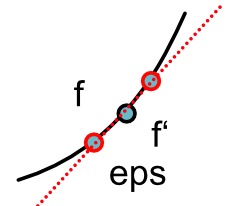
Definition of Derivative
$$f'(x) = \lim_{\epsilon \rightarrow 0} \frac{f(x + \epsilon) - f(x - \epsilon)}{2\epsilon}$$
Central Difference
Approximate derivative
$$f'(x) \approx \frac{f(x + \epsilon) - f(x-\epsilon)}{2\epsilon}$$
Approximating Derivative
Key Idea: Only need to call $f$.
In [29]:
def central_difference(f: Callable[[float], float], x: float) -> float: ...
Derivative as higher-order function
$$f(x) = ...$$ $$f'(x) = ...$$
In [30]:
def derivative(f: Callable[[float], float]) -> Callable[[float], float]:
    def f_prime(x: float) -> float:
        return minitorch.central_difference(f, x)

    return f_prime
Advanced: Mulitiple Arguments
Turn 2-argument function into 1-arg.
In [31]:
def f(x, y): ...


def f_x_prime(x: float, y: float) -> float:
    def inner(x: float) -> float:
        return f(x, y)

    return derivative(inner)(x)
Example
In [32]:
def sigmoid(x: float) -> float:
    if x >= 0:
        return 1.0 / (1.0 + math.exp(-x))
    else:
        return math.exp(x) / (1.0 + math.exp(x))


plot_function("sigmoid", sigmoid)
Example
In [33]:
sigmoid_prime = derivative(sigmoid)

plot_function("Derivative of sigmoid", sigmoid_prime)
Symbolic
- Transformation of mathematical function
- Gives full form of derivative
- Utilizes mathematical identities
Numerical
- Only requires evaluating function
- Computes derivative at a point
- Can be applied to fully black-box function
Next Class: Autodifferentiation
- Computes derivative on programs trace
- Efficient for large number of parameters
- Works directly on python code
Module-1
Module-1 Learning Objectives
- Practical understanding of derivatives
- Dive into autodifferentiation
- Parameters and their usage
Module-1: What is it?
- Numerical and symbolic derivatives
- Implement our numerical class
- Implement autodifferentiation
- Everything is scalars for now (no "gradients")