Backpropagation
The backward function tells us how to compute the derivative of one operation. The chain rule tells us how to compute the derivative of two sequential operations. In this section, we show how to use these to compute the derivative for an arbitrary series of operations.
The underlying approach we will use is a breadth-first search over the computation graph constructed by Variables and Functions. Before going over the algorithm, let's work through a specific example step by step.
Example
Assume we have Variables \(x,y\) and a Function \(h(x,y)\). We want to compute the derivatives \(h'_x(x, y)\) and \(h'_y(x, y)\).
We assume x, +, log, and exp are all implemented as ScalarFunctions which can store their history. This means that the final output Variable has constructed a graph of its history that looks like this:
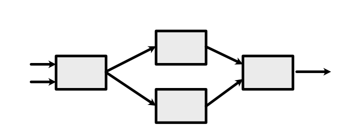
Here, starting from the left, the arrows represent Variables \(x,y\), then \(z, z\), then \(\log(z), \exp(z)\), and finally \(h(x, y)\). Forward computation proceeds left-to-right.
The chain rule tells us how to compute the derivatives. We need to apply the backward functions right-to-left until we reach the input Variables \(x,y\), which we call leaf Variables. We do this by maintaining a queue of active Variables to process. At each step, we pull a Variable from the queue, apply the chain rule to the last Function that acted on it, and then put its input Variables into the queue.
We start with only the last Variable \(h(x,y)\) in the queue (red arrow in the graph below). By default, its derivative is 1.
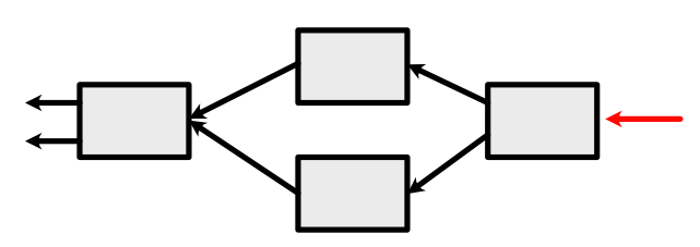
We then process it with the chain rule. This calls the backward function of +, and adds two Variables to the queue (which correspond to \(\log(z), \exp(z)\) from the forward pass).
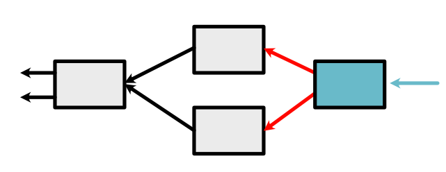
The next Variable in the queue is the top red arrow in the above graph. We pass its derivative as \(d_{out}\) in the chain rule, which adds a Variable (corresponding to \(z\): left red arrow below) to the queue.
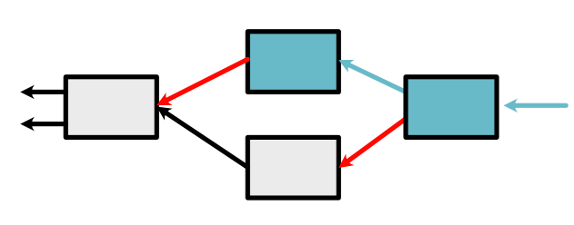
The next Variable in the queue is the bottown red arrow in the above graph. Here we have an interesting result. We have a new arrow, but it corresponds to the same Variable which is already in the queue. It is fine to have the Variable twice. Alternatively we can apply a code optimization: simply add its derivative computed at this step to its derivative computed last time. This means we only need to process one Variable in the queue.
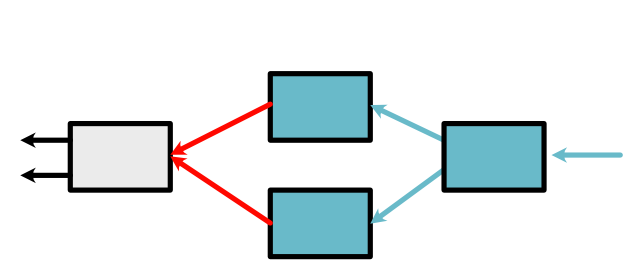
After working on this Varaible, at this point, all that is left in the queue is our leaf Variables.
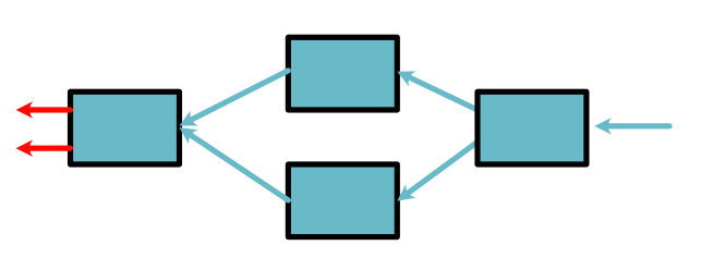
We then pull a Variable from the queue that represents an orginal leaf node, \(x\). Since each step of this process is an application of the chain rule, we can show that this final value is \(h'_x(x, y)\). The next and last step is to compute \(h'_y(x, y)\).
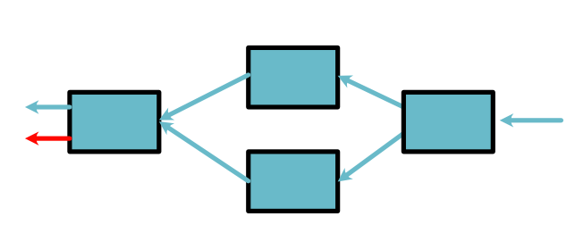
By convention, if \(x, y\) are instances of minitorch.Variable,
their derivatives are stored as:
x.derivative, y.derivative
Algorithm
This algorithm is an instance of a classic graph algorithm: breadth-first search.
As illustrated in the graph for the above example, each of the red arrows
represents
an object minitorch.VariableWithDeriv, which stores the Variable
and its current derivative
(which gets passed to \(d_{out}\) in the chain rule).
Starting from the rightmost arrow, which is passed in as an argument,
backpropagate should run the following algorithm:
Initialize a queue with the final Variable+derivative
While the queue is not empty, pull a Variable+derivative from the queue:
if the Variable is a leaf, add its final derivative (_add_deriv) and loop to (1)
if the Variable is not a leaf,
call .chain_rule on the last function that created it with derivative as \(d_{out}\)
loop through all the Variables+derivative produced by the chain rule (removing constants)
optional, if the Variable is in the queue (check .name), add to its current derivativ;
otherwise, add to the queue.
Important note: only leaf Variables should ever have non-None .derivative value. All intermediate Variables should only keep their current derivative values in the queue.