Autodifferentiation

In Tracking Variables, we have seen that ScalarFunction can be used to implement Functions on Variables. We do this by calling apply function on Variables, which then calls the underlying forward function.

(For notation, we still use capital letters to refer to our new Functions and Variables to distringuish them from Python functions and variables. We use functions to refer to mathmatical functions as well depending on the context.)

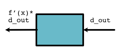
Now, we include additional information on the class which gives the derivative of the individual function. The trick behind autodifferentiation is to use a chain of function calls to compute a derivative. Just like forward calculates the function f(x), we need a backward method to provide this local derivative information.

Backward

For every Function, we need to provide a backward method to compute its derivative information. Specifically, backward computes \(f'(x) \times d_{out}\) where \(d_{out}\) is an argument passed in (discussed below).

For the simple function \(f(x) = x \times 5\), we can consult our derivative rules and get \(f'(x) = 5\). Therefore the backward is

class TimesFive(ScalarFunction):
    @staticmethod
    def forward(ctx, x):
        return x * 5

    @staticmethod
    def backward(ctx, d_out):
        f_prime = 5
        return f_prime * d_out

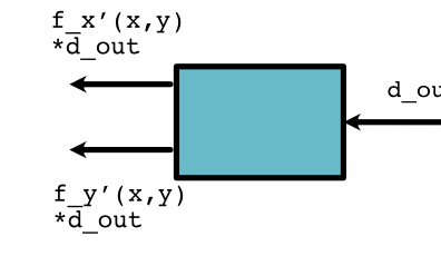
For functions that take multiple arguments, backward returns multiple deritatives with respect to each input argument. For example, if the function computes \(f(x, y)\), we need to return \(f'_x(x, y)\) and \(f'_y(x, y)\)

class Mul(ScalarFunction):
    @staticmethod
    def forward(ctx, x, y):
        # Compute f(x, y)
        pass

    @staticmethod
    def backward(ctx, d_out):
        # Compute f'_x(x, y) * d_out, f'_y(x, y) * d_out
        pass

For \(f(x, y) = x + 2 \times y\), we can consult our derivative rules again and get \(f'_x(x, y) = 1\) and \(f'_y(x, y) = 2\). Therefore the backward is

class AddTimes2(ScalarFunction):
    @staticmethod
    def forward(ctx, x, y):
        return x + 2 * y

    @staticmethod
    def backward(ctx, d_out):
        return d_out, 2 * d_out

def call(y):
     return AddTimes2.forward(None, 10, y)

plot_function("Add Times 2: x=10", call)

def d_call(y):
     return AddTimes2.backward(None, 1)[1]

plot_function("d Add Times 2: x=10", d_call)

Note that backward works a bit different than the mathematical notation. Sometimes the function for the derivative \(f'(x)\) depends directly on x; however, backward does not take \(x\) as an argument. This is not a problem for the example functions above, but things get a bit more interesting when the derivative also depends on \(x\) itself. This is where the context arguments ctx comes in.

Consider a function Square, \(f(x) = x^2\) that squares x and has derivative \(f'(x) = 2 \times x\). We write it in code as

class Square(ScalarFunction):
    @staticmethod
    def forward(ctx, x):
        ctx.save_for_backward(x)
        return x * x

    @staticmethod
    def backward(ctx, d_out):
        x = ctx.saved_values
        f_prime = 2 * x
        return f_prime * d_out

def call(x):
     # You don't need to do this manually
     # It gets called automatically in `apply`
     ctx = minitorch.Context()
     return Square.forward(ctx, x)

plot_function("Square", call)

def d_call(x):
     ctx = minitorch.Context()
     Square.forward(ctx, x)
     return Square.backward(ctx, 1)

plot_function("d Square", d_call)

This type of function requires to explicitly save anything in forward that we might need in backward. This is a code optimization that limits the amount of storage required by the computation process.

Chain Rule

Note

This section discusses implementation of the chain rule for univariate differentiation. Before reading, review the mathematical definition of Chain Rule .

The above section gives the formula for running backward on one function, but what if we need to run backward on two functions in sequence?

We can do so using the univariate chain rule:

\[f'_x(g(x)) = g'(x) \times f'_{g(x)}(g(x))\]

If the notation gets a bit hard to follow here, naming each part may be easier to understand:

\[\begin{split}\begin{eqnarray*} y &=& g(x) \\ d_{out} &=& f'(y) \\ f'_x(g(x)) &=& g'(x) \times d_{out} \\ \end{eqnarray*}\end{split}\]

The above derivative function tells us to compute the derivative of the first function (\(g\)), and then times the derivative of the second function (\(f\)) with respect to the output the first function.

Here is where the perspective of thinking of functions as boxes comes in handy:

It shows that the \(d_{out}\) multiplier passed to backward of the first box (left) should be the value returned by backward of the second box.

A similar approach works for two-argument functions:

\[\begin{split} \begin{eqnarray*} f'_x(g(x, y)) &=& g_x'(x, y) \times f'_{g(x, y)}(g(x, y)) \\ f'_y(g(x, y)) &=& g_y'(x, y) \times f'_{g(x, y)}(g(x, y)) \end{eqnarray*}\end{split}\]

Or

\[\begin{split}\begin{eqnarray*} z &=& g(x, y) \\ d_{out} &=& f'(z) \\ f'_x(g(x, y)) &=& g_x'(x, y) \times d_{out} \\ f'_y(g(x, y)) &=& g_y'(x, y) \times d_{out} \end{eqnarray*}\end{split}\]

This shows that the second box (\(f\)) does not care how many arguments the first box (\(g\)) has, as long as it passes back \(d_{out}\) which is enough for the chain rule to work.