Derivatives

Let's begin by discussing derivatives in the setting of programming. We assume that you have not seen derivatives in a while, so we will start slow and develop some notations first.

Assume we are given a function,

\[f(x) = \sin(2 x)\]

def f(x):
   return math.sin(2 * x)

plot_function("sin", f)

we can compute a function for its derivative by applying rules from univariate calculus. We will use the Lagrange notation where the derivative of a one-argument function \(f'\) as is denoted \(f'\) i.e.

\[f'(x) = 2 \times \cos(2 x)\]

def d_f(x):
   return 2 * math.cos(2 * x)

plot_function("d_sin", d_f)

When working with two-argument functions, we use subscripts to indicate which argument the derivative applies to. For example,

\[\begin{split}\begin{eqnarray*} f(x, y) &=& x + 2 y \\ f'_x(x, y) &=& 1\\ f'_y(x, y) &=& 2\\ \end{eqnarray*}\end{split}\]

We will refer to these as symbolic derivatives of the function. When available symbolic derivatives are ideal, they tell us everything we need to know about the derivative of the function.

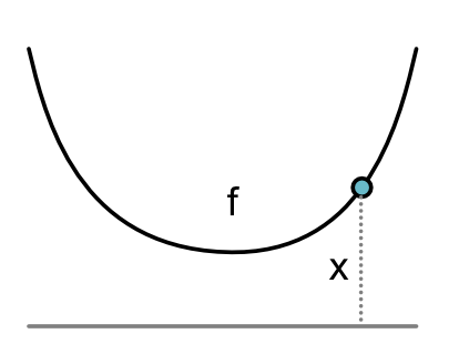
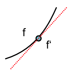
Visually, derivative functions correspond to slopes of tangent lines in 2D. Let's start with this simple function:

\[f(x) = x^2\]

Its derivative at an arbitracy input is the slope of the line tangent to that input.

\[f'(x) = 2x\]

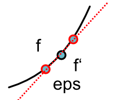
The above visual representation informally motivates an alternative approach to compute a numerical derivative. Recall one definition of the derivative function is this slope as we approach as a tangent line:

\[f'(x) = \lim_{\epsilon \rightarrow 0} \frac{f(x + \epsilon) - f(x)}{\epsilon}\]

If we set \(epsilon\) to be very small, we get an approximation of the derivative function:

\[f'(x) \approx \frac{f(x + \epsilon) - f(x)}{\epsilon}\]

Alternatively, you could imagine approaching x from the other side, which would yield a different derivative function:

\[f'(x) = \lim_{\epsilon \rightarrow 0} \frac{f(x) - f(x- \epsilon)}{\epsilon}\]

You can show that doing both simultaneously yields the best approximation (you probably proved this in high school!):

\[f'(x) \approx \frac{f(x + \epsilon) - f(x-\epsilon)}{2\epsilon}\]

The above is known as the central difference. You could find a complete description of the method here.

The key benefit of the numerical approach is that we do not need to know everything about the function: all we need is to able to compute its value under a given input. From a programming sense, this means we can approximate the derivative for any black-box function.

In implementation, it means we can write a higher-order function of the following form:

def central_difference(f, x):
    ...

Assume we are just given an arbitrary python function:

def f(x):
    "Compute some unknown function of x."
    ...

we can call central_difference(f,x) to immediately approximate the derivative of this function f on input x.

We will see that this approach is not a great way to train machine learning models, but it provides a generic alternative approach to check if your derivative functions are correct, e.g. free Property Testing.

Here are some examples of Module-0 functions with central difference applied.

plot_function("sigmoid", minitorch.operators.sigmoid)

def d_sigmoid(x):
    return minitorch.central_difference(minitorch.operators.sigmoid, x)

plot_function("Derivative of sigmoid", d_sigmoid)

plot_function("exp", minitorch.operators.exp)

def d_exp(x):
    return minitorch.central_difference(minitorch.operators.exp, x)

plot_function("Derivative of exp", d_exp)

plot_function("ReLU", minitorch.operators.relu)

def d_relu(x):
    return minitorch.central_difference(minitorch.operators.relu, x)

plot_function("Derivative of ReLU", d_relu)

def times_5(x):
    return minitorch.operators.mul(x, 5)

plot_function("Mul by 5", times_5)

def d_times_5(x):
    return minitorch.central_difference(minitorch.operators.mul, x,
    5, arg=0)

plot_function("Derivative of mul by 5", d_times_5)