Tensor Variables
Next, we consider autodifferentiation in the tensor framework. We have now moved from scalars and derivatives to vectors, matrices, and tensors. This means multivariate calculus can bring into play somewhat scary terminology. However, most of what we actually does not require complicated terminology or much technical math. In fact, except some name changes, we have already built almost everything we need in Module 1 - Auto-Differentiation.
The key idea is, just as we had Scalar and ScalarFunction, we need to construct Tensor and TensorFunction (which we just call Function). These new objects behave very similar to their counterparts:
a) Tensors cannot be operated on directly, but need to be transformed through a Function. b) Functions must implement both forward and backward. c) These transformations are tracked, which allow backpropagation through the chain rule.
All of this machinery should work out of the box.
The main new terminology to know is gradient. Just as a tensor is a multidimensional array of scalars, a gradient is a multidimensional array of derivatives for these scalars. Consider the following code:
# Assignment 1 notation
out = f(a, b, c)
out.backward()
a.derivative, b.derivative, c.derivative


# Assignment 2 notation
tensor1 = tensor(a, b, c)
out = g(tensor1)
out.backward()
# shape (3,)
tensor1.grad
The gradient of tensor1 is a tensor that holds the derivatives of each of its elements. Another place that gradients come into play is that backward no longer takes \(d_{out}\) as an argument, but now takes \(grad_{out}\) which is just a tensor consisting of all the \(d_{out}\).
Note
You will find lots of different notation for gradients and multivariate terminology. For this Module, you are supposed to ignore it and stick to everything you know about derivatives. It turns out that you can do most of machine learning without ever thinking in higher dimensions.
If you think about gradient and \(grad_{out}\) in this way (i.e. tensors of derivatives and \(d_{out}\)), then you can see how we can easily compute the gradient for tensor operations using univariate rules.
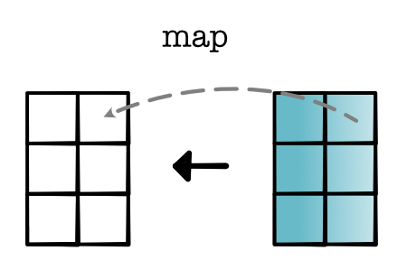
map. Given a tensor, map applies a univariate operation to each scalar position individually. For a scalar \(x\), consider computing \(g(x)\). From Module 1, we know that the derivative of \(f(g(x))\) is equal to \(g'(x) \times d_{out}\). To compute the gradient in backward, we only need to compute the derivative for each scalar position and then apply a mul map.

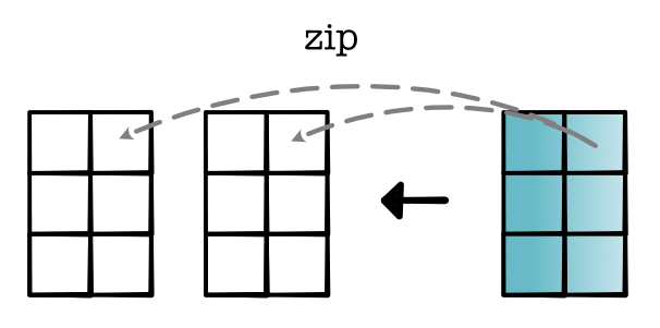
zip. Given two tensors, zip applies a binary operation to each pair of scalars. For two scalars \(x\) and \(y\), consider computing \(g(x, y)\). From Module 1, we know that the derivative of \(f(g(x, y))\) is equal to \(g_x'(x, y) \times d_{out}\) and \(g_y'(x, y) \times d_{out}\). Thus to compute the gradient, we only need to compute the derivative for each scalar position and apply a mul map.

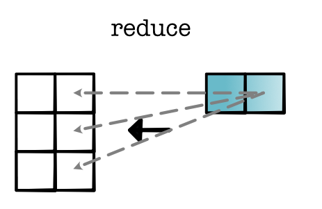
reduce. Given a tensor, reduce applies an aggregation operation to one dimension. For simplicity, let's consider sum-based reductions. For scalars \(x_1\) to \(x_n\), consider computing \(x_1 + x_2 + \ldots + x_n\). For any \(x_i\) value, the derivative is 1. Therefore, the derivative for any position computed in backward is simply \(d_{out}\). This means to compute the gradient, we only need to send \(d_{out}\) to each position. (For other reduce operations such as product, you get different expansions, which can be calculated just by taking derivatives).
