Tensors
Tensor is a fancy name for a simple concept. A tensor is a multi-dimensional array of arbitrary dimensions. It is a convenient and efficient way to hold data, which becomes much more powerful when paired with fast operators and autodifferentiation.
Tensor Shapes
So far we have focused on scalars, which correspond to 0-dimensional tensors. Next, we consider a 1-dimensional tensor (vector):
Then a 2-dimensional tensor (matrix):
In addition to its dimension (dims), other critical aspects of a tensor are its shape and size. The shape of the above vector is (5,)) and its size (i.e. number of squares in the graph) is 5. The shape of the above matrix is (2,5) and its size is 10.
A 3-dimensional tensor with shape (2, 3, 3) and size 18 looks like this:
We access an element of the tensor by tensor index notation: tensor[i] for 1-dimension, tensor[i, j] for 2-dimension, tensor[i, j, k] for 3-dimension, and so forth. For example, tensor[0, 1, 2] would give this blue cube:
Typically, we access tensors just like multi-dimensional arrays, but there are some special geometric properties that make tensors different.
First, tensors make it easy to change the order of the dimensions. For example, we can transpose the dimensions of a matrix. For a general tensor, we refer to this operation as permute. Calling permute arbitrarily reorders the dimensions of the input tensor. For example, as shown below, calling permute(1,0) on a matrix of shape (2, 5) gives a matrix of shape (5, 2). For indexing into the permuted matrix, we access elements using tensor[j, i] instead of tensor[i, j].
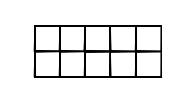
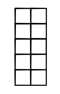
Second, tensors make it really easy to add or remove additional dimensions. Note that a matrix of shape (5, 2) can store the same amount of data as a matrix of shape (1, 5, 2), so they have the same size as shown below:

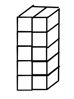
We would like to easily increase or decrease the dimension of a tensor without changing the data. We will do this with a view function: use view(1, 5, 2) for the above example. Element tensor[i, j] in the (5,2) matrix is now tensor[0, i, j] in the 3-dimensional tensor.
Critically, neither of these operations changes anything about the input tensor itself. Both view and permute are tensor tricks, i.e. operations that only modify how we look at the tensor, but not any of its data. Another way to say this is that they do not move or copy the data in any way, but only the external tensor wrapper.
Tensor Strides
Users of a Tensor library only have to be aware of the shape and
size of a tensor. However, there are important implementation details
that we need to keep track of. To make our code a bit cleaner, we
need to separate out the internal tensor data from the user-facing
tensor. In addition to the shape, minitorch.TensorData
manages tensor storage and strides:
Storage is where the core data of the tensor is kept. It is always a 1-D array of numbers of length size, no matter the dimensionality or shape of the tensor. Keeping a 1-D storage allows us to have tensors with different shapes point to the same type of underlying data.
Strides is a tuple that provides the mapping from user indexing to the position in the 1-D storage.
Strides can get a bit confusing to think about, so let's go over an example. Consider a matrix of shape (5, 2). The standard mapping is to walk left-to-right, top-to-bottom to order this matrix to the 1-D storage:
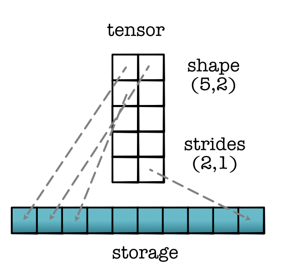
We call it contiguous mapping, since it is in the natural counting order (bigger strides left). Here the strides are \((2, 1)\). We read this as each column moves 1 step in storage and each row moves 2 steps. We can have different strides for the same shape. For instance, if we were walking top-to-bottom, left-to-right, we would have the following stride map:
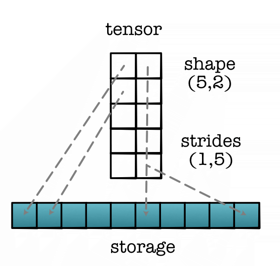
Contiguous strides are generally preferred, but non-contiguous strides can be quite useful as well. Consider transposing the above matrix and using strides (1,2):
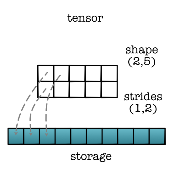
It has new strides (1,2) and new shape (5,2), in contrast to the previous (2,1) stride map on the (5,2) matrix. But notably no change in the storage. This is one of the super powers of tensors mentioned above: we can easily manipulate how we view the same underlying storage.
Strides naturally extend to higher-dimensional tensors.
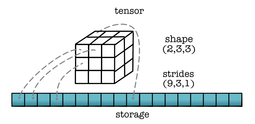
Finally, strides can be used to implement indexing into the tensor. Assuming strides are \((s_1, s_2)\) and we want to look up tensor[i, j], we can directly use strides to find its postion in the storage:
storage[s1 * i + s2 * j]
Or in general:
storage[s1 * index1 + s2 * index2 + s3 * index3 ... ]