import math
from dataclasses import dataclass

import chalk
from chalk import hcat
from colour import Color
from mt_diagrams.drawing import r
from mt_diagrams.mlprimer_draw import (
    compare,
    draw_graph,
    draw_nn_graph,
    draw_with_hard_points,
    graph,
    s,
    s1,
    s1_hard,
    s2,
    s2_hard,
    show,
    show_loss,
    split_graph,
    with_points,
)

import minitorch

chalk.set_svg_draw_height(300)
chalk.set_svg_height(300)
ML Primer
This guide is a primer on the very basics of machine learning that are necessary to complete the assignments and motivate the final system. Machine learning is a rich and well-developed field with many different models, goals, and learning settings. There are many great texts that cover all the aspects of the area in detail. This guide is not that. Our goal is to explain the minimal details of one dataset with one class of model. Specifically, this is an introduction to supervised binary classification with neural networks. The goal of this section is to learn how a basic neural network works to classify simple points.
Dataset
Supervised learning problems begin with a labeled training dataset.
We assume that we are given a set of labeled points. Each point has
two coordinates $x_1$ and $x_2$, and has a label $y$
corresponding to an O or X. For instance, here is one O labeled point:
d = hcat([split_graph([s1[0]], []), split_graph([s1[1]], [])], 0.3)
r(d, "figs/Graphs/data1.svg")

And here is an X labeled point.
d = hcat([split_graph([], [s2[0]]), split_graph([], [s2[1]])], 0.3)
r(d, "figs/Graphs/data2.svg")

It is often convenient to plot all of the points together on one set of axes.
d = split_graph(s1, s2)
r(d, "figs/Graphs/data3.svg")

Here we can see that all the X points are in the top-right and all the O points are on the bottom-left. Not all datasets is this simple, and here is another dataset where points are split up a bit more.
d = split_graph(s1_hard, s2_hard)
r(d, "figs/Graphs/data4.svg")

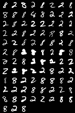
Later in the class, we will consider datasets of different forms, e.g. a dataset of handwritten numbers, where some are 8's and others are 2's:
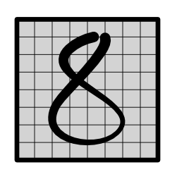
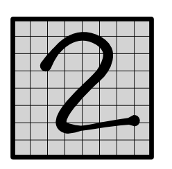
Here is an example of what this dataset looks like.
Model
Our ML system needs to specify a model that we want to the data. A model is a function that assigns labels to data points. We can specify a model in Python through its parameters and function.
@dataclass
class Linear:
    # Parameters
    w1: float
    w2: float
    b: float

    def forward(self, x1: float, x2: float) -> float:
        return self.w1 * x1 + self.w2 * x2 + self.b
This model can be written mathematically as,
$$m(x_1, x_2; w_1, w_2, b) = x_1 \times w_1 + x_2 \times w_2 + b$$.
We call it a linear model because it divides the data points up based on a line. We can visualize this be computing the "decision boundary", i.e. the areas where this function returns a positive and negative boundary.
model = Linear(1, 1, -0.9)
d = draw_graph(model)
r(d, "figs/Graphs/model1.svg")

We can overlay the simple dataset described earlier over this model. This tells us roughly how well the model fits this dataset.
d = show(model)
r(d, "figs/Graphs/incorrect.svg")

Models can take many different forms, Here is another model which has a compound form. We will discuss these types of models more below. It splits its decision into three regions (Model B).
@dataclass
class Split:
    m1: Linear
    m2: Linear

    def forward(self, x1, x2):
        return self.m1.forward(x1, x2) * self.m2.forward(x1, x2)
model_b = Split(Linear(1, 1, -1.5), Linear(1, 1, -0.5))
d = draw_graph(model_b)
r(d, "figs/Graphs/model2.svg")

Models may also have strange shapes and even disconnected regions. Any blue/red split will do, for instance (Model C):
@dataclass
class Part:
    def forward(self, x1, x2):
        return 1 if (0.0 <= x1 < 0.5 and 0.0 <= x2 < 0.6) else 0
d = draw_graph(Part())
r(d, "figs/Graphs/model3.svg")

Parameters
Once we have decided on the shape that we are using, we need a way to move between models in that class. Ideally, we would have internal knobs that alter the properties of the model.
show(Linear(1, 1, -0.5))

show(Linear(1, 1, -1))

In the case of the linear models, there are two knobs,
a. rotating the separator
model1 = Linear(1, 1, -1.0)
model2 = Linear(0.5, 1.5, -1.0)
d = compare(model1, model2)
r(d, "figs/Graphs/weight.svg")

b. changing the separator cutoff
model1 = Linear(1, 1, -1.0)
model2 = Linear(1, 1, -1.5)
d = compare(model1, model2)
r(d, "figs/Graphs/bias.svg")

Parameters are the set of numerical values that fully define a model's decisions. Parameters are critical for storing how a model acts, and necessary for producing its decision on a given data point.
Recall the functional form of the model is,
$$m(x_1, x_2; w_1, w_2, b) = x_1 \times w_1 + x_2 \times w_2 + b$$
Here $w_1, w_2, b$ are parameters, $x_1, x_2$ are the input point. The semi-colon notation indicates which arguments are for parameters and which are for data.
Our goal in this class will be to move these knobs to find the best data fit.
biases = [(i / 25.0) - 0.1 for i in range(0, 26, 5)]
d = hcat([show(Linear(1.0, 1.0, -b)) for b in biases], sep=0.5)
r(d, "figs/Graphs/knob.svg")

Loss
Observing the data, we can see that some parameters lead to good models with few classification errors,
show(Linear(1, 1, -1.0))
And some are bad and make multiple errors,
show(Linear(1, 1, -0.5))
In order to find a good model, we need to first define what good means. We
do this through a
loss function that quantifies how badly we are currently doing. A good model has small loss.
Our loss function will be based on the distance and direction of the line from each point to the decision boundary.
d = with_points(s1, s2, Linear(1, 1, -0.4))
r(d, "figs/Graphs/to_boundary.svg")

Consider a single point with different models.
This point might be classified the correct side and very far from this line (Point A, "great"):
d = with_points([s1[0]], [], Linear(1, 1, -1.5))
r(d, "figs/Graphs/pointA.svg")

Or it might be on the correct side of the line, but close to the line (Point B, "worrisome"):
d = with_points([s1[0]], [], Linear(1, 1, -1))
r(d, "figs/Graphs/pointB.svg")

Or this point might be classified on the wrong side of the line (Point C, "bad"):
d = with_points([s1[0]], [], Linear(1, 1, -0.5))
r(d, "figs/Graphs/pointC.svg")

The loss is determined based on a function of this distance. The most commonly used function (and the one we will focus on) is the sigmoid function. For strong negative inputs, it goes to zero, and for strong positive, it goes to 1. In between, it forms a smooth S-curve.
d = graph(minitorch.operators.sigmoid, width=8).scale_x(0.5)
r(d, "figs/Graphs/loss.svg")

For computational reasons, in practice we work with the log of this function. This yields a loss function that gets much worse as we move further from the decision boundary.
def point_loss(x):
    return -math.log(minitorch.operators.sigmoid(-x))
d = graph(point_loss, [], [])
r(d, "figs/Graphs/pointloss.svg")

The losses of three X points land on the following positions for the sigmoid curve. Almost zero for Point A, middle value for Point B, and nearly one for Point C.
d = graph(point_loss, [], [-2, -0.2, 1])
r(d, "figs/Graphs/pointloss2.svg")

Loss is given for the red points as well, but they are penalized in the opposite direction,
d = graph(lambda x: point_loss(-x), [-1, 0.4, 1.3], [])
r(d, "figs/Graphs/pointloss3.svg")

The total loss function $L$ for a model is the sum of each of the individual losses. Specifically,
$$L(w_1, w_2, b) = -\sum_j \log \sigma ( y^j \times m(x^j_1, x^j_2 ; w_1, w_2, b) )$$
Where $(x^j, y^j)$ are the datapoints, $\sigma$ is the sigmoid function, and multiplying by $y$ reverses the function based on the true class of the point. Here is what this looks like in code.
def full_loss(m):
    l = 0
    for x, y in zip(s.X, s.y):
        l += point_loss(-y * m.forward(*x))
    return -l


# -

# Fitting Parameters
# --------------------

# To review, the model class tells us what shapes we can consider, the parameters
# tell us the decision boundary, and the loss tells us how well the current model is doing.
#
# The last step is to produce a method for finding a good model
# given a loss function, referred to as *parameter fitting*.

# Exact parameter fitting is difficult. For all but the
# simplest models, it is a challenging task.
# This example has just 3 parameters, but some large models may have billions of parameters that need to be fit.

# We will focus on parameter fitting with *gradient
# descent*. Gradient descent works in the following manner.

# 1. Compute the loss function, $L$, for the data with the current parameters.
# 2. See how small changes to each of the parameters would change the loss.
# 3. Update the parameters with a small change in the direction that locally
#    most reduces the loss.

# Let's return to the incorrect model above.
m = Linear(1, 1, -0.5)
d = show(m)
r(d, "figs/Graphs/fit1.svg", 500)
As we noted, this model has a high loss, and we want to consider ways to "turn the knobs" of the parameters to find a better model. Let us focus on the parameter controlling the intercept.
We can consider how the loss changes with respect to just varying this parameter. It seems like the loss will go down if we move the intercept a bit.
m = Linear(1, 1, -0.55)
d = show(m)
r(d, "figs/Graphs/fit2.svg", 500)

d = show_loss(full_loss, Linear(1, 1, 0))
chalk.set_svg_height(500)
r(d, "figs/Graphs/loss.svg", 500)
d

Doing this leads to a better model.
chalk.set_svg_height(200)
We can repeat this process for the intercept as well as for all the other parameters in the model.
But how did we know how the loss function will change? For a small problem, we can move and see. But remember that machine learning models are large.
In the first module of Minitorch, we will see how to compute the direction efficiently for small problems, and then scale it up to much large models.
Neural Networks
The linear model class can be used to find good fits to the data we have considered so far, but it fails for data that splits up into multiple segments. These datasets are not linearly separable. Let us consider a very simple dataset with this property.
split_graph(s1_hard, s2_hard, show_origin=True)

Let's look at our dataset:
model = Linear(1, 1, -0.7)
draw_with_hard_points(model)

An alternative model class for this data is a neural network. Neural networks can be used to specify a much wider range of separators.
Neural networks are compound model classes that divide classification into two or more stages.
Each stage uses a linear model to seperate the data. And then an activation function to reshape it.
To see how this works consider how we might split up the datasets above. Instead of splitting all the points directly, we might first split off the left points,
yellow = Linear(-1, 0, 0.25)
ycolor = Color("#fde699")
draw_with_hard_points(yellow, ycolor, Color("white"))

And then produce another separator (green) to pull apart the red points,
green = Linear(1, 0, -0.8)
gcolor = Color("#d1e9c3")
draw_with_hard_points(green, gcolor, Color("white"))

We would like only points in the green or yellow sections to be classified as X's.
To do this, we employ an activation function that filters out only these points. This function is known as a ReLU function, which is a fancy way of saying "threshold".
$$ \text{ReLU}(z) = \begin{cases} z & z \geq 0\\ 0 & z< 0 \end{cases}$$
graph(
    minitorch.operators.relu,
    [yellow.forward(*pt) for pt in s2_hard],
    [yellow.forward(*pt) for pt in s1_hard],
    3,
    0.25,
    c=ycolor,
)

For the yellow separator, the ReLU yields the following values:
graph(
    minitorch.operators.relu,
    [green.forward(*pt) for pt in s2_hard],
    [green.forward(*pt) for pt in s1_hard],
    3,
    0.25,
    c=gcolor,
)

Basically the right X's are thresholed to positive values and the other O's and X's are 0.
Finally yellow and green become our new $x_1, x_2$. Since all the O's are now at the origin it is very easy to separate out the space.
draw_nn_graph(green, yellow)

Looking back at the original model, this process appears like it has produced two lines to pull apart the data.
@dataclass
class MLP:
    lin1: Linear
    lin2: Linear
    final: Linear

    def forward(self, x1, x2):
        x1_1 = minitorch.operators.relu(self.lin1.forward(x1, x2))
        x2_1 = minitorch.operators.relu(self.lin2.forward(x1, x2))
        return self.final.forward(x1_1, x2_1)
mlp = MLP(green, yellow, Linear(3, 3, -0.3))
draw_with_hard_points(mlp)

d = draw_with_hard_points(mlp)
r(d, "figs/Graphs/hard.svg")
Mathematically we can think of the transformed data as values $h_1, h_2$ which we get from applying separators with different parameters to the original data. The final prediction then applies a separator to $h_1, h_2$.
\begin{eqnarray*} h_ 1 &=& \text{ReLU}(x_1 \times w^0_1 + x_2 \times w^0_2 + b^0) \\ h_ 2 &=& \text{ReLU}(x_1 \times w^1_1 + x_2 \times w^1_2 + b^1)\\ m(x_1, x_2) &=& h_1 \times w_1 + h_2 \times w_2 + b \end{eqnarray*}
Here $w_1, w_2, w^0_1, w^0_2, w^1_1, w^1_2, b, b^0, b^1$ are all parameters. We have gained more flexible models, at the cost of now needing to fit many more parameters to the data.
This neural network will be the main focus for the first couple models. It appears quite simple, but fitting it effectively will require building up systems infrastructure. Once we have this infrastructure, though, we will be able to easily support most modern neural network models.